Exercise: Population Dynamics

Question 1

You are studying a closed population of beetles consisting of 3000 individuals. You register 400 births and 150 deaths during one month. Calculate r and lambda and predict the population size after 6 months.

Answer: We assume 400 births and 150 deaths within a month. Build a model based on a projection interval of one month. Then \[ \begin{align} N_{t+1} &= N_t + B - D = 3000 + 400 - 150 = 3250\\ \lambda &= \frac{N_{t+1}}{N_{t}} = \frac{3250}{3000} = 1.0833\\ r &= \ln \lambda = \ln(1.0833) = 0.08\\ N_6 &= 3000* \exp(0.08*6) = 3000*1.0833^6= 4848 \end{align} \] Thus, after six month we expect 4848 beetles.

Question 2

You estimate the size of a flatworm population to be the following at five consecutive days: 100, 158, 315, 398 and 794 individuals. Plot the natural logarithm (i.e., to the base e) of the population size and estimate r. You can plot the data by hand on a piece of paper, or by using EXCEL or R.

Answer: Start by taking the natural logarithm of the five population estimates, resulting in 4.605, 5.063, 5.753, 5.986, and 6.677. Plot these as a function of time (days).

Draw a straight line through the data points. There are exact mathematical methods, for example, the method of least squares (linear regression) that can be executed in R or Excel. Here you can see the R-code for doing this.

x <- 1:5
y <- c(4.605, 5.063, 5.753, 5.986, 6.677)

plot(x, y, xlab = "day", ylab = "population size")
linear.regression <- lm(y ~ x)
linear.regression

## 
## Call:
## lm(formula = y ~ x)
## 
## Coefficients:
## (Intercept)            x  
##      4.0967       0.5067

abline(linear.regression)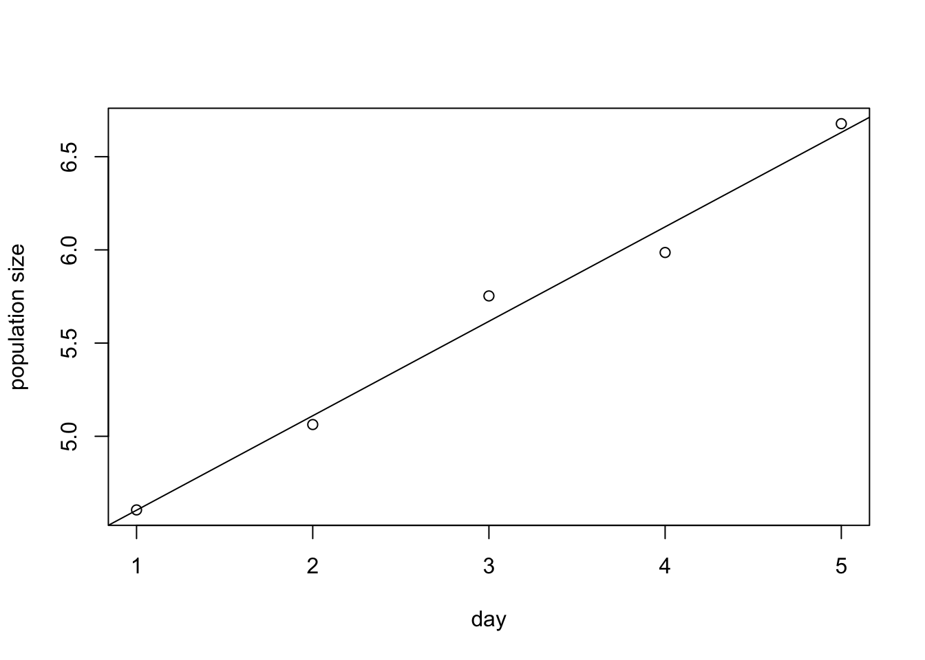

The regression analysis also shows the value for the slope, namely \(0.5067\). This slope is equal to the population growth rate \(r\).

For the purpose of this exercise it is sufficient to draw the line with the “naked eye” and estimate its slope by dividing the change in \(y\) by the change in \(x\), \(\Delta y/\Delta x\).

Question 3

An isolated population of elk (a species of deer) in Washington state increased from 1975 to 1993 as follows:

\[ \begin{align*} 1975 &\,\,\,\,\, 8 & 1986 &\,\,\,\,\, 68 \\ 1976 &\,\,\,\,\, 13 & 1987 &\,\,\,\,\, 67 \\ 1977 &\,\,\,\,\, 14 & 1988 &\,\,\,\,\, 72 \\ 1979 &\,\,\,\,\, 15 & 1989 &\,\,\,\,\, 79 \\ 1981 &\,\,\,\,\, 20 & 1990 &\,\,\,\,\, 94 \\ 1982 &\,\,\,\,\, 21 & 1991 &\,\,\,\,\, 110 \\ 1983 &\,\,\,\,\, 27 & 1992 &\,\,\,\,\, 146 \\ 1984 &\,\,\,\,\, 40 & 1993 &\,\,\,\,\, 179 \\ 1985 &\,\,\,\,\, 54 && \end{align*} \] Plot these data. What shape of population growth is shown by these data? Could one fit the logistic equation to these data? Use a discrete-time model to calculate the net reproductive ratio \(\lambda\) for this population.

Answer:

x <- c(1975, 1976, 1977, 1978, 1979, 1980, 1981, 1982, 1983, 1984, 1985, 1986, 1987, 1988, 1989, 1990, 1991, 1992, 1993)
y <- c(8, 13, 14, NA, 15, NA, 20, 21, 27, 40, 54, 68, 67, 72, 79, 94, 110, 146, 179)

plot(x, y, xlab = "year", ylab = "population size")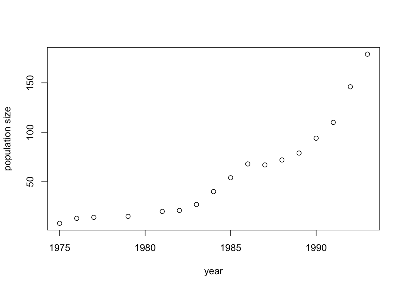

There is no evidence for the curve to level off around an equilibrium K. Rather, the elk population seems to grow exponentially.

We can use the same method as under Q2 to calculate \(\lambda\):

lny <- log(y)
plot(x, lny, xlab = "day", ylab = "population size")
linear.regression <- lm(lny ~ x)
linear.regression

## 
## Call:
## lm(formula = lny ~ x)
## 
## Coefficients:
## (Intercept)            x  
##   -320.8056       0.1635

abline(linear.regression)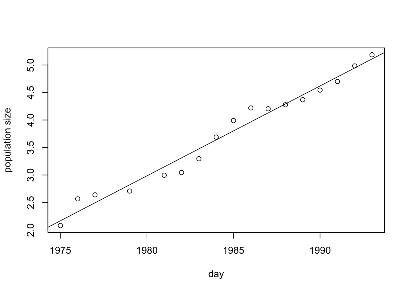

Thus \(r=0.1635\), and \[ \lambda=\exp(r)=\exp(0.1635)=1.177625. \]

Alternatively, solving for r can done as follows: \[ \begin{align} N_t &= N_0 \lambda^{t}\\ \lambda^{t} &= \frac{N_t}{N_0}\\ \lambda &=\left(\frac{N_t}{N_0}\right)^{\frac{1}{t}}=\sqrt[^{t}]{\frac{N_t}{N_0}}\\ \lambda &= \sqrt[^{18}]{\frac{179}{8}} = \sqrt[^{18}]{22.375}\approx1.19 \end{align} \]

Question 4

Suppose that a butterfly population shows logistic growth with K = 500 and r = 0.1 individuals/(individuals*month). What is the maximal growth rate for this population?

Answer: Recall that the growth rate of a logistically growing population is highest when population size equals N = K/2. Since K = 500 this population will grow fastest at N = 500/2 = 250. Then \[ \frac{\mathrm{d}N}{\mathrm{d}t} = rN\left(1-\frac{N}{K}\right) \Longrightarrow 0.1*250\left(1-\frac{250}{500}\right)= 12.5. \] Thus, the maximal population growth rate equals 12.5 individuals per month.

Question 5

A fisher is maximizing their fishing yield by maintaining a population of logistically growing lake trout at the density where the population growth rate is fastest. For the population in question, this occurs at a density of 500 individuals. Predict the realized population growth rate after the population has been stocked with an additional 600 fish. Assume that for the trout r=0.005 individuals/(individual*day).

Answer: The fact that this logistically growing population is growing fastest at K/2=500 individuals implies that K = 1000. With 600 fish added the new population size equals 1100. Then \[ \frac{\mathrm{d}N}{\mathrm{d}t} = rN\left(1-\frac{N}{K}\right) \Longrightarrow 0.005*1100\left(1-\frac{1100}{1000}\right) = -0.55. \] Thus, the growth rate equals -0.55 fish per day. The growth rate is negative because the additional stock pushes the population above its carrying capacity.